Triangles
Triangles are one of the most important primitives that make up the virtual space of 3D modeling. Triangles can be easily stored by the locations of its three vertices. Many 3D model file types do exactly that and reconstruct a full surface or object by specifying different combinations of three vertices that make up the different triangular faces on a 3D object. Furthermore, triangular shapes can benefit from barycentric coordinate system that allow any point on the triangle to be interpolated as a linear combination of the three vertex values
If we treat the coordinates of each vertex as a position vector inside an original coordinate system, a non-orthogonal coordinate system can be constructed for the plane in which the triangle lies in. The two major axes of such a coordinate system are the difference vectors of two of the vertices from the same vertex.
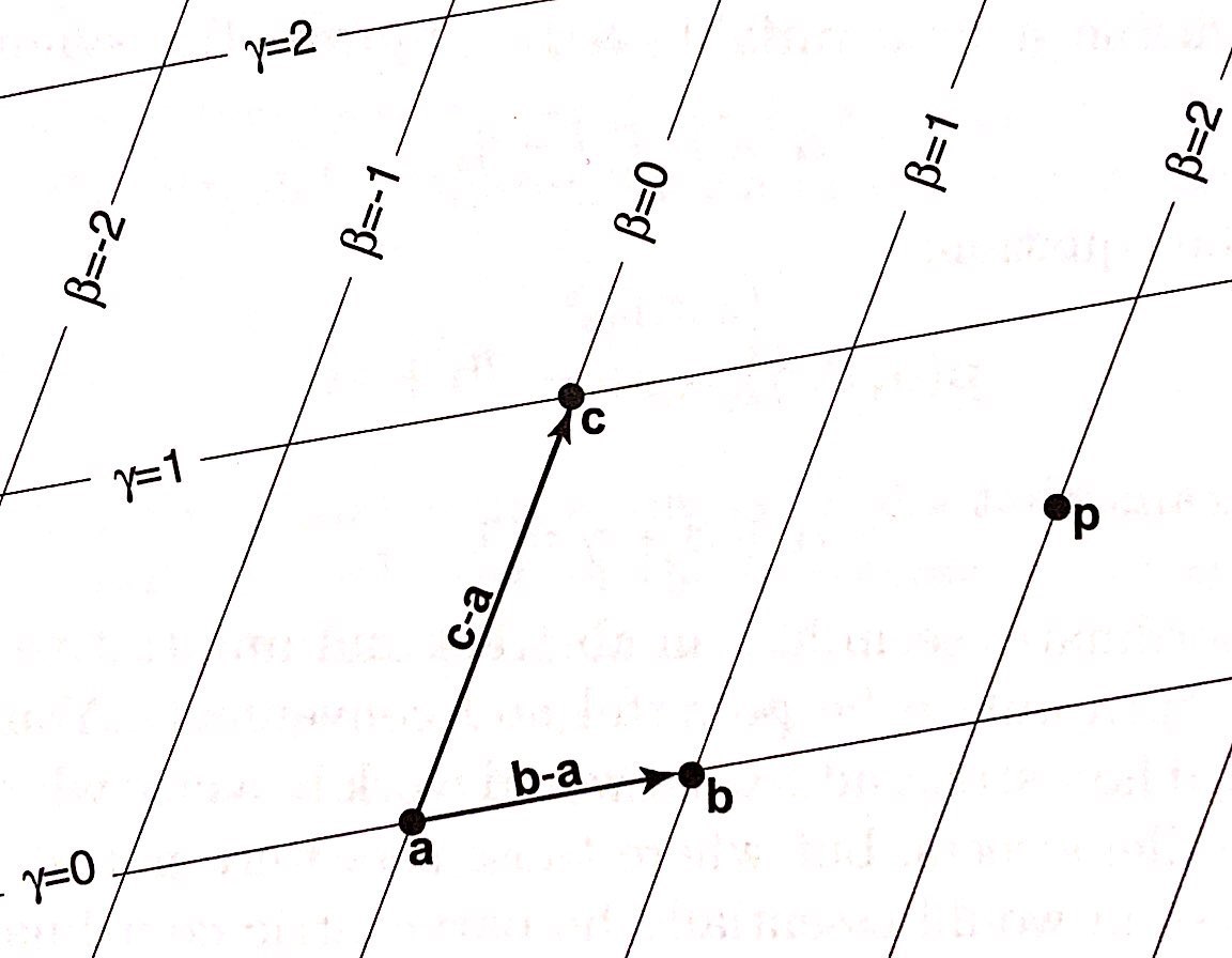
With barycentric coordinate systems, the coordinates of every point on the triangle can be easily interpolated. The same applies to the colors. Given $\mathbf{c_0}$, $\mathbf{c_1}$ and $\mathbf{c_2}$ at the three vertices of the triangle, the color at a given point ($\alpha, \beta, \gamma$) is given by
$\mathbf{c(\alpha, \beta, \gamma)} = \alpha\mathbf{c_0} + \beta\mathbf{c_1} + \gamma\mathbf{c_2}$
As shown, the information regarding a whole triangle, its shape and color, can be easily derived from the basic information regarding only three points, proving triangles to be a powerful primitive that is used to efficiently construct 3D shapes.
To gain a basic understanding of the graphics pipeline, we first implemented a simulation in the high-level programming language Python. In this simulation, we read in data regarding the positions of several vertices that combine to form triangular faces before transforming the image and ultimately outputting a bitmap describing the image.
Object Parsing and Transformation
To begin, we read in an object file that typically specifies the vertices and the faces present in the 3D object. The example below is that of a tetrahedron in .OBJ format. Each line that starts with "V" specifies the coordinates of a given vertex, and each that starts with "F" specifies the three vertices that makes up a triangular face.
Lighting
Naturally, we must next calculate how lighting affects the appearance of the 3D object. To find the intensity of the light falling on a given point on the object, and thus the brightness of the object at that point, we dot a lighting vector $\mathbf{l}$ with the vector normal to each of the object's surfaces. We compute this normal vector $\hat{\mathbf{n}}$ by taking the cross product of two of the face's edge vectors and normalizing by dividing by the magnitude of this cross product.
$\hat{\mathbf{n}} = \frac{\mathbf{e_0}\times\mathbf{e_1}}{\mid\mathbf{e_0}\times\mathbf{e_1}\mid}$
The brightness of the face is thus proportional to $\hat{\mathbf{n}}\cdot\mathbf{l}$. In order to speed up the development of our simulation and avoid stalling our progress to learn computer graphics, we did not implement this step in our Python code.
Projection
In order to project the 3D object onto the screen space available, we must perform another series of matrix multiplications. We perform a perspective projection by imagining the actual position of the object behind the screen and some focal point, ideally where the user's eyes are, in front of the screen and projecting the image onto screen such that the projected outlines of the image converge to the focal point. In our example, we perform these projections as follows, dividing only by powers of two to allow division by bit-shifting:
$screen-[x,y,z] = ((([x,y,z]/4)+1)/2)*screen-[width,height,depth]$
This operation can also be implemented in multiple stage of matrix multiplication.
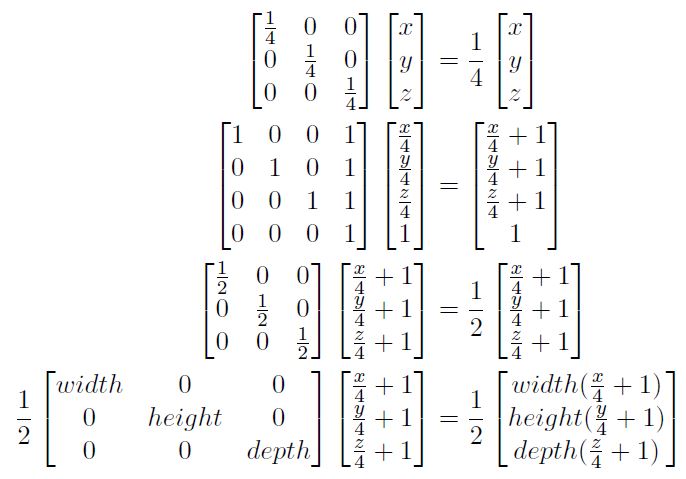
Through this conversion, we made a majority of our operations into matrix multiplication, which would allow large parallelism in hardware and its reuse.
Rasterization
Usually, it is necessary to interpolate all the discrete points on each face through barycentric coordinates to make a non-hollow surface. However, for development simplicity, we chose to only interpolate the three edges between two of the three vertices in a face in the 3D screen space. The interpolation is done using Bresenham's line algorithm. Two buffers are essential for then projecting the 3D screen space onto a 2D grey-scale screen/bitmap. As the two dimensional grey-scale bitmap can be seen as a matrix, a Z buffer and a Color buffer can be each seen as a matrix who entries are the value the buffers for a given pixel (x, y) within that 2D space. For each pixel in the 2D space, the Z buffer initiates with the furthest Z screen space. Only when a point in the 3D screen space with the same x and y value has a smaller Z value would Z(x, y) updates to that smaller Z value and allow the Color buffer to update to the new color value. In this way, a geometry that is behind and obstructed would be painted over rather painting over the geometries in front of it, which causes incorrect display. The Python code for the two buffer operation is shown below.