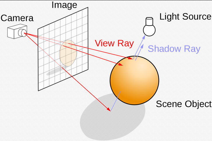
When people normally think of the path a light travels, one would start from the light source with a light ray. The light ray would proceed to run into an object and reflect off the surface. Finally, those light rays would end up in your eyes and allow you to perceive light the way you do. However, this is not the process that takes place in the computer graphics world. Even with a single point as the light source, the light rays from the single point would go out in every direction inside the virtual 3D space. Some of them may be heading in a direction of no return while others would be simply blocked by objects in the way. In neither of the cases would the light enter your eye. As those light rays become irrelevant how you perceive the world, the elimination of such rays would significantly reduce the amount of computation done. The way to know whether we care about a light ray, not surprisingly, begins its journey at “the eye”, or the viewing point inside the virtual 3D space. As the ray cast into the model space gets reflected off of a surface and finally reaches a light source, the patch of object surface would then be computationally rendered with the added effects of light.
Ray tracing provides a multitude of benefits over traditional raster graphics. The reason that ray tracing is only now becoming possible in real time is that it is extremely computationally expensive. In 1980, Turner Whitted of Bell Labs calculated that between 75% and 95% of the time ray tracing required was dedicated to calculating the intersection points of rays with objects in the scene. As a result, methods of simplifying and accelerating that calculation have been devised and, in combination with Moore's Law, have enabled the advent of realtime ray tracing.
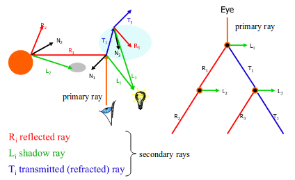
In ray tracing, it is important to understand the types of rays we are casting. First, we have primary rays, which go from the viewpoint to the ray's nearest intersection point. Next, we have secondary rays, which begin at the intersection points of the primary rays. These rays exist because of reflection, refraction, and shadows. In the case of shadow rays, rays are sent from the nearest intersection point of the primary ray with the scene towards the light sources in the scene. If the shadow rays reach the light source unobstructed, the intersection point in question can be considered to be in the shadow of some object.
Ray-triangle Intersection Test
As mentioned in the raster graphics, triangles made up one of the most important primitives that are used to construct a 3D object thanks to its low-cost long-term storage and versatile geometric property. A ray cast onto a triangle based 3D model is bound to hit one of the triangles. Determining the exact triangle that insects with the light ray is thus an unavoidable task in the ray tracing world.
From barycentric coordinate system, we know that a point, given triangle $\mathbf{ABC}$, can be expressed as
$\mathbf{p}(\gamma, \beta) = \gamma(\mathbf{c}-\mathbf{a})+\beta(\mathbf{b}-\mathbf{a})+\mathbf{a}$
At the same time, the light ray we cast from a viewing point $\mathbf{e}$ through a pixel point $\mathbf{s}$ is given by
$\mathbf{r}=\mathbf{e}+\mathbf{d}t$
$with \mathbf{d} = \mathbf{s}-\mathbf{e}$
We can find if there is an intersection between the plane of the triangle and the light ray and where by equating the two equations and solve for $\beta, \gamma$, and $t$
$\mathbf{e}+\mathbf{d}t = \gamma(\mathbf{c}-\mathbf{a})+\beta(\mathbf{b}-\mathbf{a})+\mathbf{a}$
The vector equation can be broken up as three equations
$x_e+x_dt = x_a+\beta(x_b-x_a)+\gamma(x_c-x_a)$
$y_e+y_dt = y_a+\beta(y_b-y_a)+\gamma(y_c-y_a)$
$z_e+z_dt = z_a+\beta(z_b-z_a)+\gamma(z_c-z_a)$
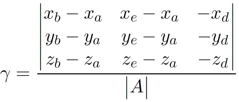
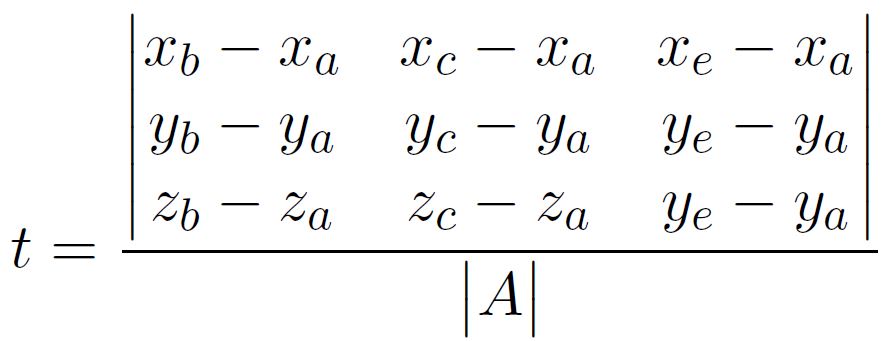
which can rewritten in matrix form as the following
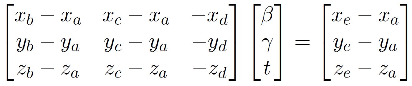
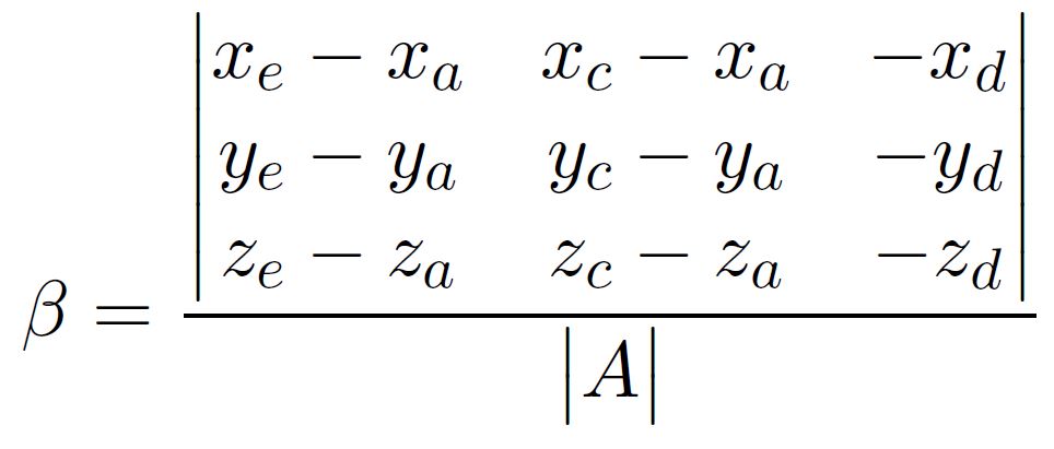
With Cramer’s rule, we know that for an matrix multiplication $\mathbf{A}\vec{x}=\vec{b}$ assuming $\mathbf{A}$ invertible, the solution to $x_i$, which is the ith entry of the unknown vector, is given by
$x_i = \frac{det[\mathbf{A_i}]}{det[\mathbf{A}]}$
where $\mathbf{A_i}$ stands for the matrix $\mathbf{A}$ with ith column replaced with $\vec{b}$.
Nonetheless, for he given point of intersection to sit within the triangle, we would need the solutions to abide by the following
$\gamma + \beta < 1$
$\gamma > 0$
$\beta > 0$
$t_{min} < t < t_{max}$
$t_{min}$ and $t_{max}$ specify the block region within which the triangles are located. Such regions is discussed in the next section
Bounding Box
Ray-triangle intersection tests become expensive as a direct test would require checking every single triangle to determine the relevant triangles. The size of the problem grows linearly with the number of triangles within a 3D scene and quickly become not manageable. Various techniques can be employed to achieve sublinear performance. “Divide and conquer” with bounding boxes is one of the efficient ways to achieve the performance. We first take a look at 2D bounding box.
For a 2D bounding box, its four edges can be represented as
$x = x_{min}$
$x = x_{max}$
$y = y_{min}$
$y = y_{max}$
As a light ray is parameterized as $f=x_e+tx_d$, finding the t at which the light ray intersects with a given ray is
$t_{xmin} = \frac{x_{min}-x_e}{x_d}$
$t_{xmax} = \frac{x_{max}-x_e}{x_d}$
$t_{ymin} = \frac{y_{min}-y_e}{y_d}$
$t_{ymax} = \frac{y_{max}-y_e}{y_d}}$
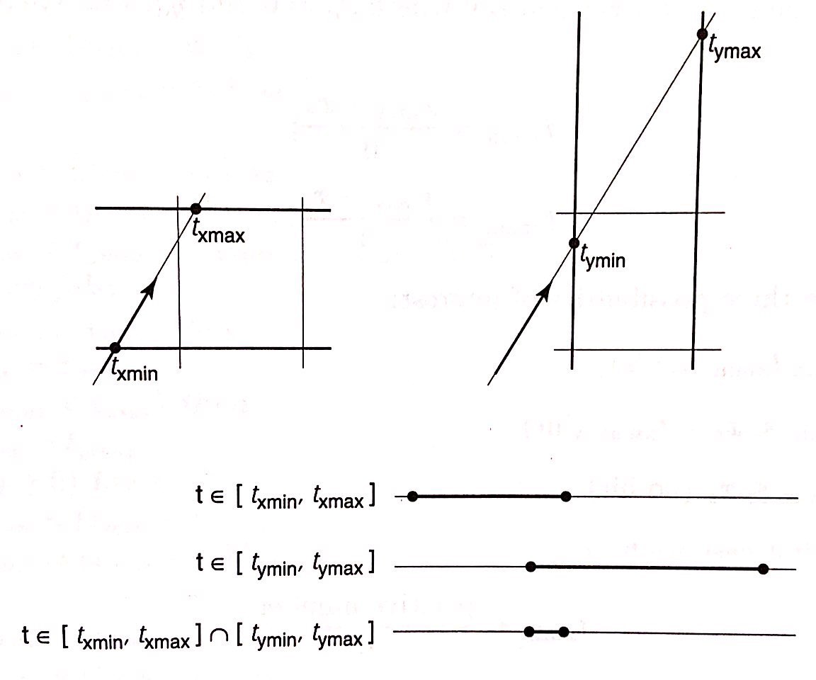
The only way for the light ray to intersect a box is to fulfill the following condition
$[t_{xmin}, t_{xmax}]\cup[t_{ymin}, t_{ymax}] \ne \emptyset$
Which makes sense as if the minimum of one is larger than the maximum of the other there will not be any intersection. The following picture also illustrate this principle well.
The bounding box in 3D easily extend the same principle into a higher dimension.
$[t_{xmin}, t_{xmax}]\cup[t_{ymin}, t_{ymax}] \cup[t_{zmin}, t_{zmax}]\ne \emptyset$
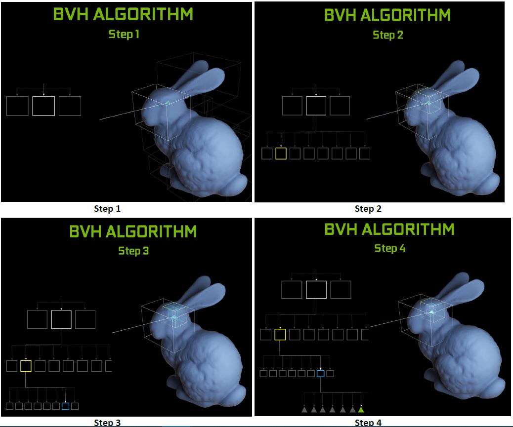
Bounding Volume Hierarchy
In order to effectively implement this method of looking at bounding boxes, we can create a structure known as a Bounding Volume Hierarchy (BVH). A BVH is a tree structure that contains subtrees and, at its lowest levels, a set of basic primitives such as triangles. This structure exploits coherence in a scene in order to break the primitives of a scene into groups. These groups, for example, might contain the entire scene at the highest level, similar objects at the next level, a singular object at the next, and primitives at the last. The BVH we will utilize relies on an object hierarchy, which is more robust over time than a spatial hierarchy in dynamic scenes. It also contributes to better hardware performance, as it can reject bounding volumes irrelevant to a given ray extremely quickly.
It is important to consider the shape of the bounding volumes as well. To simplify and reduce the number of calculations, loosely constrained bounding volumes may seem the best option, but many rays that hit these volumes will still miss the object or primitive within them. In contrast, if the bounding volume for an object is simply that object, we will waste fewer calculations but need to perform more calculations overall. As a result, we generally select volumes somewhere between these two extremes, such as parallelopipeds or spheres.
When optimizing a BVH, the intersection point of a ray with a bounding volume is actually irrelevant. Instead, all we care about is whether or not the ray intersects the volume. It then becomes important to search and store the BVH in an efficient manner. In this vein, ray casting algorithms tend to perform a depth-first traversal of the BVH. Moreover, one efficient approach to storing a BVH is to maintain a tree where each node contains a reference to the left-most child, the right sibling, and the parent node. This organization allows us to store a skip node, which contains the node to which we redirect our search if we arrive at a leaf or miss a bounding volume. This ensures better memory usage; though more information is stored in the tree, the nodes are stored in the order they are accessed in, providing memory coherence. [Smits 1999] Another way to improve memory performance is to cache the most recently hit object and check that object and the surrounding scene first with the next rays, as they will likely be directed in quite similar directions to the last ray.
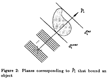
Ray packets are another technique for optimizing the process of ray tracing. To minimize the hardware necessary to construct these packets, we utilize ray packet sizes that are powers of two. Additionally, we may approach the problem of computing ray-box overlap from the perspective of Kay and Kajiya's slabs algorithm. This algorithm essentially relies on breaking bounding volumes up into sets of planes, or slabs. These slabs are the space between two planes, such that the one plane is $d_{near}$ units from the origin and one is $d_{far}$ units from the origin, with the planes being defined by a vector normal to each surface of the bounding volume, the volume itself an intersection of bounding slabs. We then compute the intersection of a ray with a slab by computing its intersection with both slabs to compute an interval for the intersection. If we then compute the intersection of the intervals, we can compute the intersection of the ray with a bounding volume. Many solutions to the problem of ray-axis-aligned-bounding-box intersection tests are variants on this slab test.
Denoising And Filtering
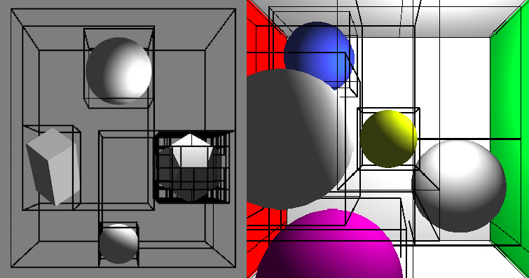
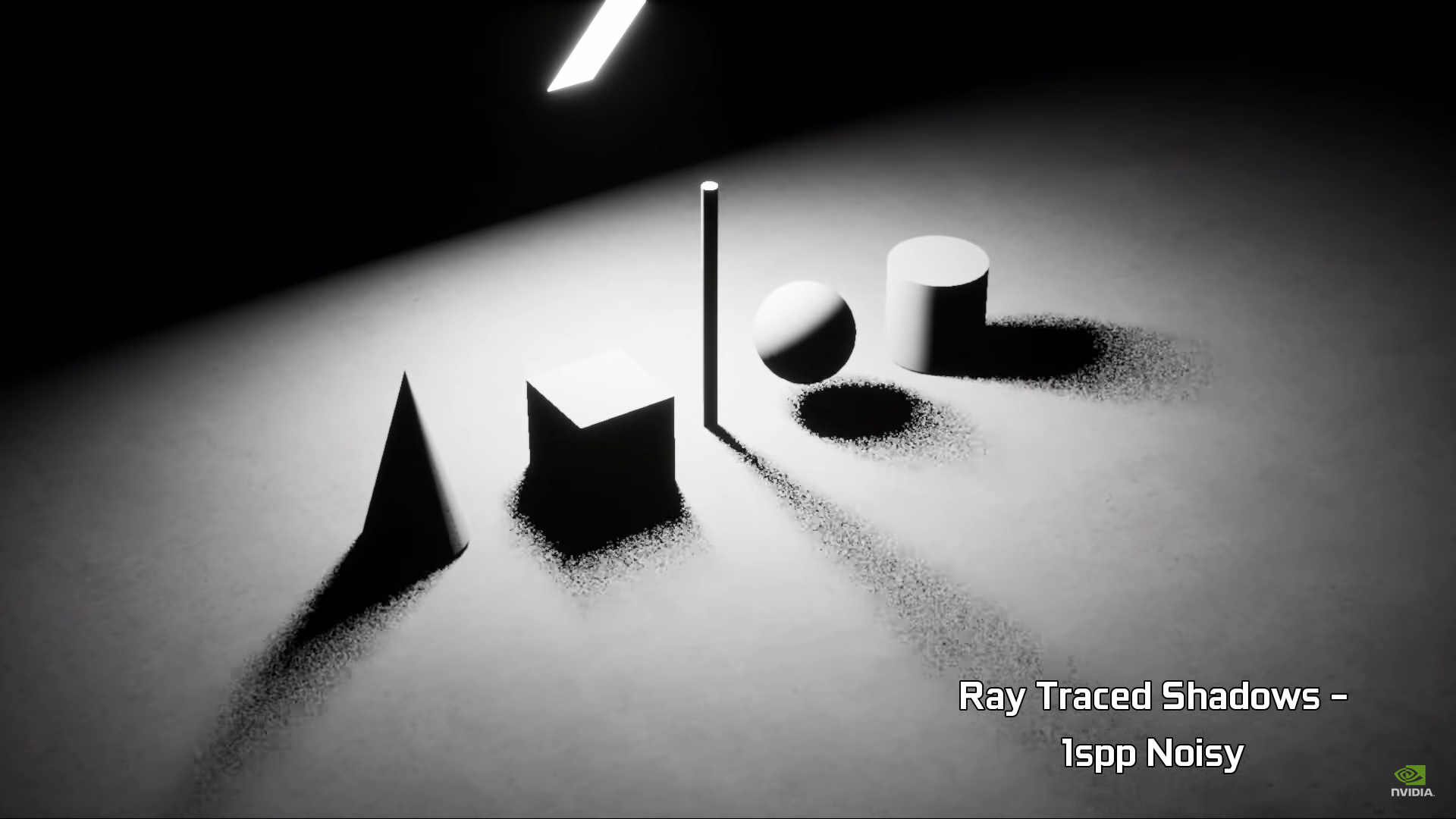
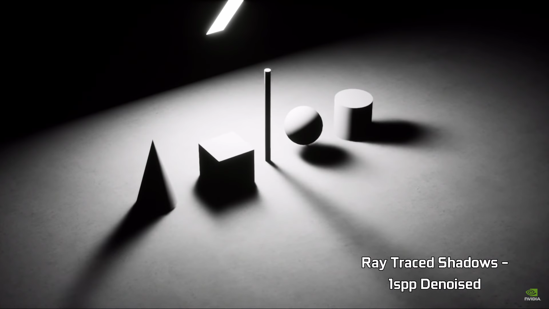
Despite the enormous amount of calculation that went into tracing rays back to objects it hits and the light sources it originates from, real time ray tracing alone is still insufficient in generating a photo realistic image due to the small number of rays per pixel. Various filtering and denoising techniques are empolyed to generate better images. The differences in quality in various rendering techniques and the presence of post processing are shown below.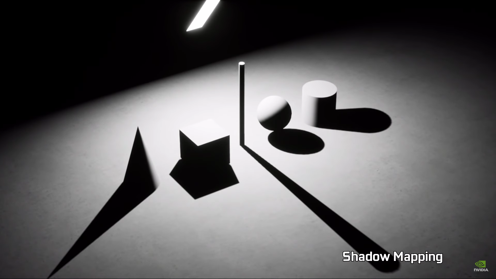
In order to achieve fast denoising, engineers rely upon rather complex algorithms, such as Monte Carlo methods, to generate the most realistic image with low sample rates. Monte Carlo methods comprise a group of algorithms that rely on repeated random sampling to compute numerical results. In other words, they take advantage of randomness in order to solve problems. Thus, they are fundamentally able to exploit the parallelism present in graphics processing hardware necessary for ray tracing and denoising. Though they require a non-trivial amount of computational power, they work effectively because they are naturally parallel. One example of a Monte Carlo method is path tracing, or Monte Carlo ray tracing, which randomly traces potential light paths in order to render a scene. To be precise, there are actually two different forms of ray tracing that utilize Monte Carlo methods. First, we can cast a ray from the viewpoint through each pixel before casting random rays from the intersection point of that primary ray. Second, we can cast many primary rays per pixel, but only trace one secondary ray for each. Combining both of these, we can achieve a useful model for randomly sampling rays in a scene. By repeatedly sampling the light paths for a pixel, the pixel value should eventually converge on the correct value and allow the scene to be rendered.
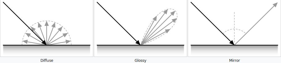
In conjunction with these algorithms that rely on randomness, the output of the ray tracing acceleration hardware is constantly being filtered in order to provide frames that effectively display glossy reflections, area light-soft shadows, and ambient occlusion. Researchers have yet to converge on a single methodology for this filtering, but many publications indicate a reliance on cross-bilateral filters and bidirectional reflectance distribution functions (BRDF). Though we will not dive into the math of these filters, we can provide some background on their inner workings. For instance, BRDFs indicate how light reflects off of a surface based on its matte or glossy nature. We can combine these BRDFs with the corresponding Fresnel coefficients, which describe the reflection and transmission of light, in order to create an accurate model of light's interaction with different surfaces. In An Efficient Denoising Algorithm for Global Illumination, the authors utilize the Lambertian reflectance approximation as well, which defines surfaces with brightnesses that do not vary regardless of viewing angle. They also indicate that by approximating the reflectance vectors of some rays given that the matte-ness and thus the angle of reflection stays relatively near constant over areas the display coherence in a scene, we can factor terms out of the expression for the Monte Carlo integrator in order to calculate the brightness of a surface in a way that will allow us to reconstruct images with less computation than earlier methods required. A series of bilateral filter can then be applied to smooth image or video frames by calculating the intensity of each pixel with the weighted average of the surrounding pixels.